Chapter 7 Reporting: tables
Scenario. Lucy seems intrigued your presentation on Australia’s sales. Now, she wants to review the sales difference (growth) for Product Category and Sub Category between year 2015 and 2016. She wants to be able to filter the report by all the options available, including Customer Gender and Age Group.
Load libraries
library(tidyverse, warn.conflicts = F)
library(scales)
library(formattable)
library(htmlwidgets)
library(sparkline)
Load data for this lab:
my_data <- readRDS("./data/processing/data4week3.rds")
str(my_data)
## Classes 'tbl_df', 'tbl' and 'data.frame': 113036 obs. of 19 variables:
## $ Date : POSIXct, format: "2013-11-26" "2015-11-26" ...
## $ Year : num 2013 2015 2014 2016 2014 ...
## $ Month : num 11 11 3 3 5 5 5 5 2 2 ...
## $ Customer ID : num 11019 11019 11039 11039 11046 ...
## $ Customer Age : num 19 19 49 49 47 47 47 47 35 35 ...
## $ Age Group : chr "Youth" "Youth" "Adults" "Adults" ...
## $ Customer Gender : chr "M" "M" "M" "M" ...
## $ Country : chr "Canada" "Canada" "Australia" "Australia" ...
## $ State : chr "British Columbia" "British Columbia" "New South Wales" "New South Wales" ...
## $ Product Category: chr "Accessories" "Accessories" "Accessories" "Accessories" ...
## $ Sub Category : chr "Bike Racks" "Bike Racks" "Bike Racks" "Bike Racks" ...
## $ Product : chr "Hitch Rack - 4-Bike" "Hitch Rack - 4-Bike" "Hitch Rack - 4-Bike" "Hitch Rack - 4-Bike" ...
## $ Frame Size : num NA NA NA NA NA NA NA NA NA NA ...
## $ Order Quantity : num 8 8 23 20 4 5 4 2 22 21 ...
## $ Unit Cost : num 45 45 45 45 45 45 45 45 45 45 ...
## $ Unit Price : num 120 120 120 120 120 120 120 120 120 120 ...
## $ Cost : num 360 360 1035 900 180 ...
## $ Revenue : num 950 950 2401 2088 418 ...
## $ Profit : num 590 590 1366 1188 238 ...In this Lab we’ll be review the sales difference (growth) for Product Category and Sub Category between year 2015 and 2016. So, we will create two type of reports. One with the sales for each year and the other with the % Change in Revenue from year to year. Each report is a cross-tabular format with Product Categories and Sub categories on the rows and year on the columns, with Sum of Revenue as the aggregate data. Also we will create chart representation for each report.
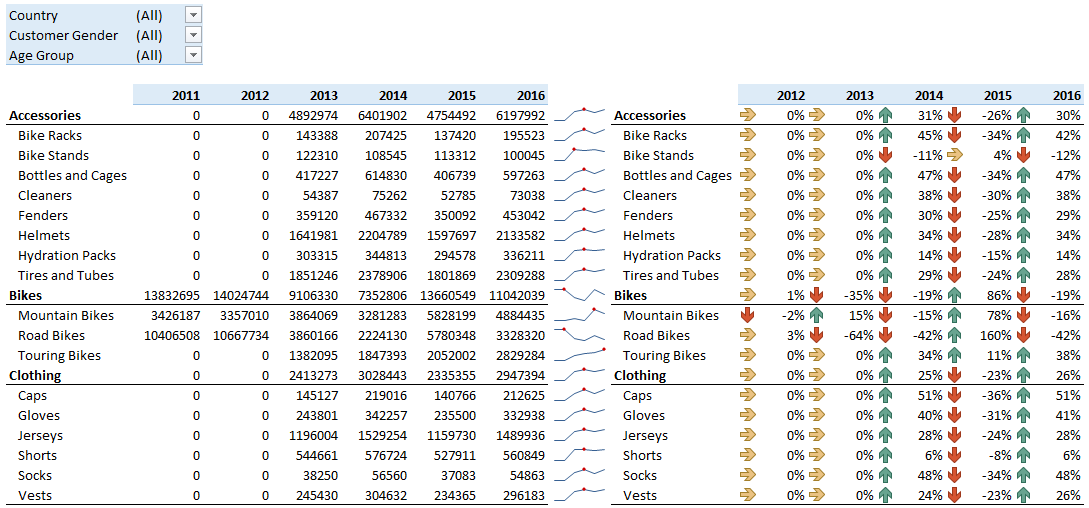
Let’s start! First, create two reports just like on picture below
For this task we’re going to use such packages as formattable and sparklines. Also we’ll include external css file for styling our tables.
7.1 Helper functions for type 1 report
7.1.1 Count totals for Product Category
product_total <- function(df) {
  df %>%
    group_by(`Product Category`, Year) %>%
    summarise(Total = sum(Revenue)) %>%
    mutate(Margin = (Total - lag(Total)) / Total) %>%
    ungroup() %>%
    mutate(`Sub Category` = `Product Category`) %>%
    select(`Product Category`, `Sub Category`, everything())
}| Product Category | Sub Category | Year | Total | Margin |
|---|---|---|---|---|
| Accessories | Accessories | 2013 | 3384215 | NA |
| Accessories | Accessories | 2014 | 4293592 | 0.2117987 |
| Accessories | Accessories | 2015 | 3285954 | -0.3066501 |
| Accessories | Accessories | 2016 | 4154231 | 0.2090103 |
| Bikes | Bikes | 2011 | 8964888 | NA |
| Bikes | Bikes | 2012 | 9175983 | 0.0230052 |
| Bikes | Bikes | 2013 | 9858787 | 0.0692584 |
| Bikes | Bikes | 2014 | 7611243 | -0.2952926 |
| Bikes | Bikes | 2015 | 14799083 | 0.4856950 |
| Bikes | Bikes | 2016 | 11372150 | -0.3013443 |
| Clothing | Clothing | 2013 | 1997035 | NA |
| Clothing | Clothing | 2014 | 2247889 | 0.1115954 |
| Clothing | Clothing | 2015 | 1938954 | -0.1593308 |
| Clothing | Clothing | 2016 | 2187004 | 0.1134200 |
7.1.2 List of unique product in Product Category
uniq_product <- function(df) {
  unique(df$`Product Category`)
}
my_data %>% uniq_product()
## [1] "Accessories" "Clothing" "Bikes"7.1.3 Count totals for Sub Category:
sub_total <- function(df) {
  df %>%
  group_by(`Product Category`, `Sub Category`, Year) %>%
  summarise(Total = sum(Revenue)) %>%
  mutate(Margin = (Total - lag(Total)) / Total) %>%
  ungroup()
}| Product Category | Sub Category | Year | Total | Margin |
|---|---|---|---|---|
| Accessories | Bike Racks | 2013 | 112605 | NA |
| Accessories | Bike Racks | 2014 | 152966 | 0.2638560 |
| Accessories | Bike Racks | 2015 | 107813 | -0.4188085 |
| Accessories | Bike Racks | 2016 | 144416 | 0.2534553 |
| Accessories | Bike Stands | 2013 | 95396 | NA |
| Accessories | Bike Stands | 2014 | 83148 | -0.1473036 |
| Accessories | Bike Stands | 2015 | 88822 | 0.0638806 |
| Accessories | Bike Stands | 2016 | 76709 | -0.1579085 |
| Accessories | Bottles and Cages | 2013 | 292535 | NA |
| Accessories | Bottles and Cages | 2014 | 422000 | 0.3067891 |
7.1.4 Prepare report_1
report_1 <- function(df) {
  bind_rows(product_total(df), sub_total(df)) %>%
  select(-Margin) %>%
  group_by(`Product Category`, Year) %>%
  spread(key = Year, value = Total) %>%
  group_by(`Product Category`) %>%
  arrange(desc(`2016`), .by_group = TRUE) %>%
  ungroup() %>%
  select(-`Product Category`) %>%
  mutate_if(is.numeric, formattable::comma, digits = 0)
}
my_data %>% report_1
## # A tibble: 20 x 7
## `Sub Category` `2011` `2012` `2013`
## <chr> <S3: formattable> <S3: formattable> <S3: formattable>
## 1 Accessories NA NA 3,384,215
## 2 Helmets NA NA 1,285,031
## 3 Tires and Tubes NA NA 1,033,740
## 4 Bottles and Cages NA NA 292,535
## 5 Fenders NA NA 284,577
## 6 Hydration Packs NA NA 237,491
## 7 Bike Racks NA NA 112,605
## 8 Bike Stands NA NA 95,396
## 9 Cleaners NA NA 42,840
## 10 Bikes 8,964,888 9,175,983 9,858,787
## 11 Road Bikes 6,766,618 6,993,130 4,836,352
## 12 Mountain Bikes 2,198,270 2,182,853 3,732,841
## 13 Touring Bikes NA NA 1,289,594
## 14 Clothing NA NA 1,997,035
## 15 Jerseys NA NA 956,093
## 16 Shorts NA NA 447,464
## 17 Gloves NA NA 191,818
## 18 Vests NA NA 251,704
## 19 Caps NA NA 117,068
## 20 Socks NA NA 32,888
## # ... with 3 more variables: `2014` <S3: formattable>, `2015` <S3:
## # formattable>, `2016` <S3: formattable>7.1.5 Define function that makes sparklines in formattable object
my_sparkline <- function(x){
  as.character(
    htmltools::as.tags(
      sparkline(x) # we can add any chart type!
    )
  )
}
7.1.6 Make tibble with sparklines as html-widgets:
sparkl_df <- function(df) {
  report_1(df) %>%
  nest(`2011`:`2016`, .key = 'Sparkl') %>%
  mutate_at('Sparkl', map, as.numeric, my_sparkline) %>%
  mutate_at('Sparkl', map, my_sparkline)
}
7.1.7 Add sparklines objects to report_1:
report_1_sparkl <- function(df) {
  bind_cols(report_1(df), sparkl_df(df) %>%
                        select(Sparkl))
}
my_data %>% report_1_sparkl
## # A tibble: 20 x 8
## `Sub Category` `2011` `2012` `2013`
## <chr> <S3: formattable> <S3: formattable> <S3: formattable>
## 1 Accessories NA NA 3,384,215
## 2 Helmets NA NA 1,285,031
## 3 Tires and Tubes NA NA 1,033,740
## 4 Bottles and Cages NA NA 292,535
## 5 Fenders NA NA 284,577
## 6 Hydration Packs NA NA 237,491
## 7 Bike Racks NA NA 112,605
## 8 Bike Stands NA NA 95,396
## 9 Cleaners NA NA 42,840
## 10 Bikes 8,964,888 9,175,983 9,858,787
## 11 Road Bikes 6,766,618 6,993,130 4,836,352
## 12 Mountain Bikes 2,198,270 2,182,853 3,732,841
## 13 Touring Bikes NA NA 1,289,594
## 14 Clothing NA NA 1,997,035
## 15 Jerseys NA NA 956,093
## 16 Shorts NA NA 447,464
## 17 Gloves NA NA 191,818
## 18 Vests NA NA 251,704
## 19 Caps NA NA 117,068
## 20 Socks NA NA 32,888
## # ... with 4 more variables: `2014` <S3: formattable>, `2015` <S3:
## # formattable>, `2016` <S3: formattable>, Sparkl <list>7.1.8 Final table for the first report
report_1_table <- function(df) {
  formattable(report_1_sparkl(df),
    align = c("l", "r", "r", "r", "r", "r", "r"), table.attr = "class=\'my_table\'",
    list(
      area(, `2011`:`2016`) ~ color_tile("#FFFF00", "#FF0000"),
      `Sub Category` = formatter("span",
               style = x ~ ifelse(x %in% uniq_product(df),
                            style(font.weight = "bold"),
                            style(padding.left = "0.25cm"))
                                )
        )
    ) %>%
  formattable::as.htmlwidget() %>%
  htmltools::tagList() %>%
  htmltools::attachDependencies(htmlwidgets:::widget_dependencies("sparkline","sparkline")) %>%
  htmltools::browsable()
}
my_data %>% report_1_table()
7.2 Helper functions for report type 2
7.2.1 Calculate changes in totals by year for product category
report_2 <- function(df) {
  bind_rows(product_total(df), sub_total(df)) %>%
  select(-Total) %>%
  group_by(`Product Category`, Year) %>%
  spread(key = Year, value = Margin) %>%
  ungroup() %>%
  arrange(match(`Sub Category`, report_1(df)$`Sub Category`)) %>%
  select(-`Product Category`, -`2011`) %>%
  mutate_if(is.numeric, formattable::percent, digits = 1)
}
my_data %>% report_2
## # A tibble: 20 x 6
## `Sub Category` `2012` `2013` `2014`
## <chr> <S3: formattable> <S3: formattable> <S3: formattable>
## 1 Accessories NA NA 21.2%
## 2 Helmets NA NA 21.1%
## 3 Tires and Tubes NA NA 22.7%
## 4 Bottles and Cages NA NA 30.7%
## 5 Fenders NA NA 18.0%
## 6 Hydration Packs NA NA 10.2%
## 7 Bike Racks NA NA 26.4%
## 8 Bike Stands NA NA -14.7%
## 9 Cleaners NA NA 26.2%
## 10 Bikes 2.3% 6.9% -29.5%
## 11 Road Bikes 3.2% -44.6% -60.3%
## 12 Mountain Bikes -0.7% 41.5% -25.1%
## 13 Touring Bikes NA NA 20.0%
## 14 Clothing NA NA 11.2%
## 15 Jerseys NA NA 15.4%
## 16 Shorts NA NA -2.7%
## 17 Gloves NA NA 23.4%
## 18 Vests NA NA -10.1%
## 19 Caps NA NA 27.5%
## 20 Socks NA NA 21.4%
## # ... with 2 more variables: `2015` <S3: formattable>, `2016` <S3:
## # formattable>7.2.2 Final table for the second report
report_2_table <- function(df) {
  formattable(report_2(df), align = c("l", "l", "l", "l", "l", "l"),
    table.attr = "class=\'my_table\'",
    list(
      area(, `2012`:`2016`) ~ formatter("span",
        style = x ~ style(color = ifelse(x < 0 , "red", "green")),
                x ~ icontext(ifelse(x < 0, "arrow-down", "arrow-up"), formattable::percent(x, digits = 1))),
     `Sub Category` = formatter("span",
                style = x ~ ifelse(x %in% uniq_product(df),
                           style(font.weight = "bold"),
                           style(padding.left = "0.25cm")
                                  )
                                )
      )
  )
}
my_data %>% report_2_table()| Sub Category | 2012 | 2013 | 2014 | 2015 | 2016 |
|---|---|---|---|---|---|
| Accessories | NA | NA | 21.2% | -30.7% | 20.9% |
| Helmets | NA | NA | 21.1% | -30.3% | 20.7% |
| Tires and Tubes | NA | NA | 22.7% | -33.1% | 22.5% |
| Bottles and Cages | NA | NA | 30.7% | -48.0% | 30.4% |
| Fenders | NA | NA | 18.0% | -25.2% | 17.6% |
| Hydration Packs | NA | NA | 10.2% | -14.6% | 10.4% |
| Bike Racks | NA | NA | 26.4% | -41.9% | 25.3% |
| Bike Stands | NA | NA | -14.7% | 6.4% | -15.8% |
| Cleaners | NA | NA | 26.2% | -39.6% | 26.3% |
| Bikes | 2.3% | 6.9% | -29.5% | 48.6% | -30.1% |
| Road Bikes | 3.2% | -44.6% | -60.3% | 58.6% | -62.9% |
| Mountain Bikes | -0.7% | 41.5% | -25.1% | 46.6% | -25.6% |
| Touring Bikes | NA | NA | 20.0% | 16.9% | 21.1% |
| Clothing | NA | NA | 11.2% | -15.9% | 11.3% |
| Jerseys | NA | NA | 15.4% | -21.8% | 15.7% |
| Shorts | NA | NA | -2.7% | -0.4% | -2.3% |
| Gloves | NA | NA | 23.4% | -35.2% | 23.9% |
| Vests | NA | NA | -10.1% | 7.3% | -11.1% |
| Caps | NA | NA | 27.5% | -42.0% | 27.5% |
| Socks | NA | NA | 21.4% | -30.9% | 21.2% |
7.3 Questions
7.3.1 Without applying any filter, which year does the Accessories category have negative growth?
Answer: 2015
7.3.2 Filter the reports for youth age group. Which two years do the accessories category have negative growth?
Report 1
my_data %>%
  filter(`Age Group` == "Youth") %>%
report_1_table()my_data %>%
filter(`Age Group` == "Youth") %>%
report_2_table()| Sub Category | 2012 | 2013 | 2014 | 2015 | 2016 |
|---|---|---|---|---|---|
| Accessories | NA | NA | -7.8% | 4.9% | -8.9% |
| Tires and Tubes | NA | NA | 13.7% | -18.0% | 13.1% |
| Helmets | NA | NA | -16.6% | 12.0% | -18.3% |
| Bottles and Cages | NA | NA | 30.3% | -45.9% | 29.1% |
| Fenders | NA | NA | -39.2% | 25.9% | -37.9% |
| Hydration Packs | NA | NA | -106.0% | 49.6% | -110.6% |
| Cleaners | NA | NA | 15.1% | -21.7% | 15.9% |
| Bike Stands | NA | NA | -144.7% | 57.6% | -185.4% |
| Bike Racks | NA | NA | -53.4% | 32.2% | -44.9% |
| Bikes | -1.3% | -8.9% | -140.8% | 72.8% | -143.7% |
| Road Bikes | -0.9% | -73.4% | -127.8% | 71.7% | -142.6% |
| Mountain Bikes | -2.7% | 41.8% | -169.9% | 75.2% | -152.9% |
| Touring Bikes | NA | NA | -113.8% | 69.6% | -120.1% |
| Clothing | NA | NA | -92.8% | 47.0% | -95.0% |
| Jerseys | NA | NA | -59.1% | 35.6% | -59.6% |
| Gloves | NA | NA | 18.6% | -25.5% | 17.5% |
| Caps | NA | NA | 1.7% | -5.1% | 3.1% |
| Shorts | NA | NA | -612.6% | 85.8% | -661.4% |
| Vests | NA | NA | -246.9% | 70.1% | -245.8% |
| Socks | NA | NA | -9.9% | 8.3% | -16.4% |
Answer: 2014, 2016
7.4 Without applying any filter, which two years do the bikes category have negative growth?
Answer: 2014, 2016
7.5 Filter the report for Australia. Which year do the bikes category have the highest growth?
Report 1
my_data %>%
  filter(Country == "Australia") %>%
report_1_table()my_data %>%
filter(Country == "Australia") %>%
report_2_table()| Sub Category | 2012 | 2013 | 2014 | 2015 | 2016 |
|---|---|---|---|---|---|
| Accessories | NA | NA | 18.9% | -26.7% | 18.5% |
| Helmets | NA | NA | 18.5% | -25.9% | 18.0% |
| Tires and Tubes | NA | NA | 24.7% | -36.3% | 24.4% |
| Bottles and Cages | NA | NA | 29.6% | -45.8% | 28.8% |
| Hydration Packs | NA | NA | -11.7% | 7.7% | -12.0% |
| Fenders | NA | NA | 9.6% | -13.0% | 9.4% |
| Bike Racks | NA | NA | 60.9% | -170.0% | 60.3% |
| Bike Stands | NA | NA | -39.0% | 24.9% | -38.1% |
| Cleaners | NA | NA | 35.6% | -58.2% | 36.0% |
| Bikes | 1.1% | 16.2% | -84.2% | 64.6% | -88.5% |
| Road Bikes | 2.5% | -4.6% | -84.5% | 64.6% | -85.7% |
| Mountain Bikes | -2.1% | 25.4% | -126.4% | 71.3% | -139.0% |
| Touring Bikes | NA | NA | -11.3% | 41.3% | -13.7% |
| Clothing | NA | NA | -14.7% | 11.7% | -17.1% |
| Jerseys | NA | NA | -7.2% | 4.6% | -8.7% |
| Shorts | NA | NA | -35.0% | 23.8% | -36.3% |
| Gloves | NA | NA | 21.9% | -33.3% | 22.8% |
| Vests | NA | NA | -98.3% | 51.1% | -109.4% |
| Caps | NA | NA | 26.3% | -39.4% | 25.2% |
| Socks | NA | NA | 21.7% | -29.7% | 20.9% |
Answer: 2015
7.6 Keep the Australia filter. In the year that bikes sales have the highest growth (previous question), which sub category of bikes has the highest growth?
Answer: Mounting Bikes, 71%