Chapter 9 Join data from different sources

Scenario. Lastly, Lucy wants to have more information about the customer demographics in addition to the already available age and gender. Since your data has Customer ID for each row, you can “connect” these rows with your customer demographics database. Your customer demographics is stored in file “Customer_demographics.txt”.

Load necessary libraries

library(tidyverse)
library(RColorBrewer)
library(scales)

Load data for Lab8:

my_data <- readRDS("./data/processing/data4week3.rds")
glimpse(my_data)

## Observations: 113,036
## Variables: 19
## $ Date               <dttm> 2013-11-26, 2015-11-26, 2014-03-23, 2016-0...
## $ Year               <dbl> 2013, 2015, 2014, 2016, 2014, 2016, 2014, 2...
## $ Month              <dbl> 11, 11, 3, 3, 5, 5, 5, 5, 2, 2, 7, 7, 7, 7,...
## $ `Customer ID`      <dbl> 11019, 11019, 11039, 11039, 11046, 11046, 1...
## $ `Customer Age`     <dbl> 19, 19, 49, 49, 47, 47, 47, 47, 35, 35, 32,...
## $ `Age Group`        <chr> "Youth", "Youth", "Adults", "Adults", "Adul...
## $ `Customer Gender`  <chr> "M", "M", "M", "M", "F", "F", "F", "F", "M"...
## $ Country            <chr> "Canada", "Canada", "Australia", "Australia...
## $ State              <chr> "British Columbia", "British Columbia", "Ne...
## $ `Product Category` <chr> "Accessories", "Accessories", "Accessories"...
## $ `Sub Category`     <chr> "Bike Racks", "Bike Racks", "Bike Racks", "...
## $ Product            <chr> "Hitch Rack - 4-Bike", "Hitch Rack - 4-Bike...
## $ `Frame Size`       <dbl> NA, NA, NA, NA, NA, NA, NA, NA, NA, NA, NA,...
## $ `Order Quantity`   <dbl> 8, 8, 23, 20, 4, 5, 4, 2, 22, 21, 8, 8, 7, ...
## $ `Unit Cost`        <dbl> 45, 45, 45, 45, 45, 45, 45, 45, 45, 45, 45,...
## $ `Unit Price`       <dbl> 120, 120, 120, 120, 120, 120, 120, 120, 120...
## $ Cost               <dbl> 360, 360, 1035, 900, 180, 225, 180, 90, 990...
## $ Revenue            <dbl> 950, 950, 2401, 2088, 418, 522, 379, 190, 2...
## $ Profit             <dbl> 590, 590, 1366, 1188, 238, 297, 199, 100, 1...

Customer demographics database:

add_data <- read.table("./data/raw/Customer_demographics.txt", sep = ",", header = T) %>%
    as_data_frame()
glimpse(add_data)

## Observations: 18,484
## Variables: 7
## $ ID               <int> 1, 2, 3, 4, 5, 6, 7, 8, 9, 10, 11, 12, 13, 14...
## $ Customer.ID      <int> 11000, 11001, 11002, 11003, 11004, 11005, 110...
## $ MaritalStatus    <fctr> M, S, M, S, S, S, S, M, S, S, S, M, M, M, S,...
## $ YearlyIncome     <int> 90000, 60000, 60000, 70000, 80000, 70000, 700...
## $ TotalChildren    <int> 2, 3, 3, 0, 5, 0, 0, 3, 4, 0, 0, 4, 2, 2, 3, ...
## $ EnglishEducation <fctr> Bachelors, Bachelors, Bachelors, Bachelors, ...
## $ HouseOwnerFlag   <lgl> TRUE, FALSE, TRUE, FALSE, TRUE, TRUE, TRUE, T...

---

9.1 For those customers who bought bikes, what are the top three (bought the most quantity) customer profiles (marital status and number of children)?

ans_1 <- my_data %>%
    select(`Customer ID`, `Order Quantity`, `Product Category`) %>%
    left_join(add_data %>%
                  select(Customer.ID, MaritalStatus, TotalChildren), c("Customer ID" = "Customer.ID")) %>% 
    filter(`Product Category` == "Bikes") %>%
    group_by(MaritalStatus, TotalChildren) %>%
    summarise(`Total Order` = sum(`Order Quantity`)) %>%
    arrange(desc(`Total Order`)) %>% 
    ungroup()
kable(ans_1)

MaritalStatus	TotalChildren	Total Order
S	0	6733
M	1	5487
M	2	4029
S	2	3873
M	0	3845
S	1	2729
M	3	2375
M	4	2009
S	3	1802
S	4	1550
M	5	1145
S	5	834

ggplot(ans_1, aes(x = factor(TotalChildren), y = `Total Order`, fill = factor(MaritalStatus))) +
    geom_bar(stat = "identity", position = position_dodge(0.55), width = 0.5) +
    scale_y_continuous(breaks = seq(0, 7e3, 1e3), expand = c(0.01, 0),
                       limits = c(0, 7e3), oob = scales::squish) +
    labs(x = "Total Children", fill = "Marital\nStatus") +
    theme(plot.title = element_text(face = "bold", size = 14, hjust = 0.3),
          panel.background = element_rect(fill = "white"),
          legend.title = element_text(colour = "black", size = 10, face = "bold"),
          legend.text = element_text(colour = "black", size = 10, face = "bold"),
          legend.position = c(.95, .90),
          legend.background = element_rect(color = "black"),
          axis.line = element_line(colour = "black"),
          axis.text = element_text(size = 11, colour = "black"),
          axis.title = element_text(size = 12, face = "bold"))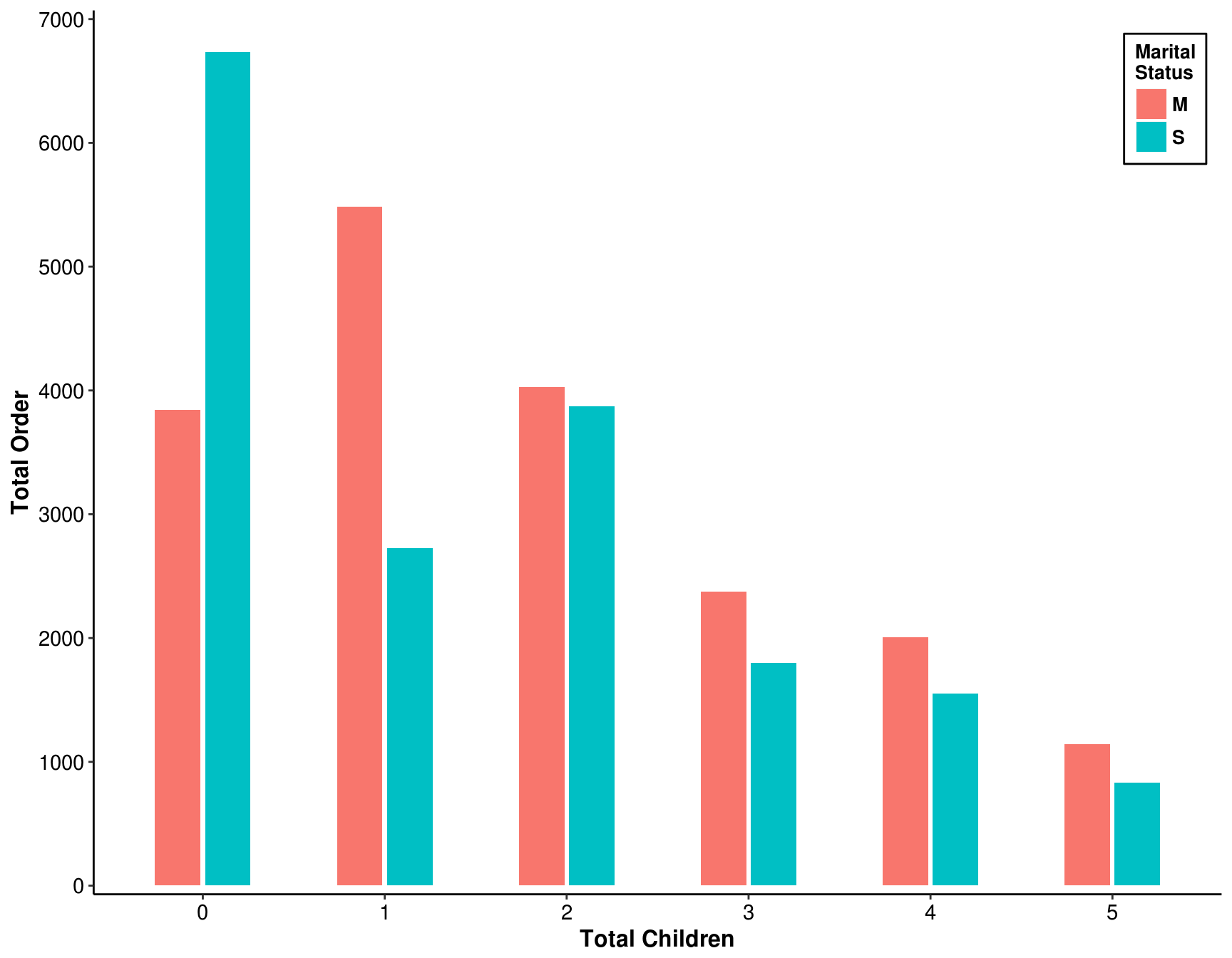

Answer: 1. Single without child 2. Married with one child 3. Married with two children

---

Now, replace the MaritalStatus and TotalChildren fields with the YearlyIncome field from the Customer_demographic table.

9.2 For those customers who bought bikes, what are the top three (bought the most quantity) income brackets? (Rank from highest to Lowest)

ans_2 <- my_data %>%
    select(`Customer ID`, `Order Quantity`, `Product Category`) %>%
    left_join(add_data %>%
                  select(Customer.ID, YearlyIncome), c("Customer ID" = "Customer.ID")) %>% 
    filter(`Product Category` == "Bikes") %>%
    group_by(YearlyIncome)%>%
    summarise(`Total Quantity` = sum(`Order Quantity`)) %>%
    arrange(desc(`Total Quantity`)) %>% 
    ungroup()
kable(ans_2)

YearlyIncome	Total Quantity
40000	5573
60000	5288
70000	5125
30000	4992
20000	2817
80000	2333
90000	2037
10000	1861
130000	1439
110000	1310
50000	1038
100000	898
120000	819
170000	324
150000	305
160000	252

`Yearly Income` <- reorder(ans_2$YearlyIncome, -ans_2$`Total Quantity`)
ggplot(ans_2, aes(x = `Yearly Income`, y = `Total Quantity`)) +
    geom_bar(stat = "identity", width = 0.5, fill = "tomato2") +
    scale_y_continuous(breaks = seq(0, 6e3, by = 1e3), expand = c(0.01, 0),
                       limits = c(0, 6e3), oob = scales::squish) +
    scale_x_discrete(expand = c(0.01, 0), labels = paste0("$", prettyNum(`Yearly Income`, big.mark = "'"))) + 
    theme_classic() +
    theme(axis.text.x = element_text(angle = 65, vjust = 1.0, hjust = 1.0),
          axis.text = element_text(size = 11, colour = "black"),
          axis.title = element_text(size = 12, face = "bold"))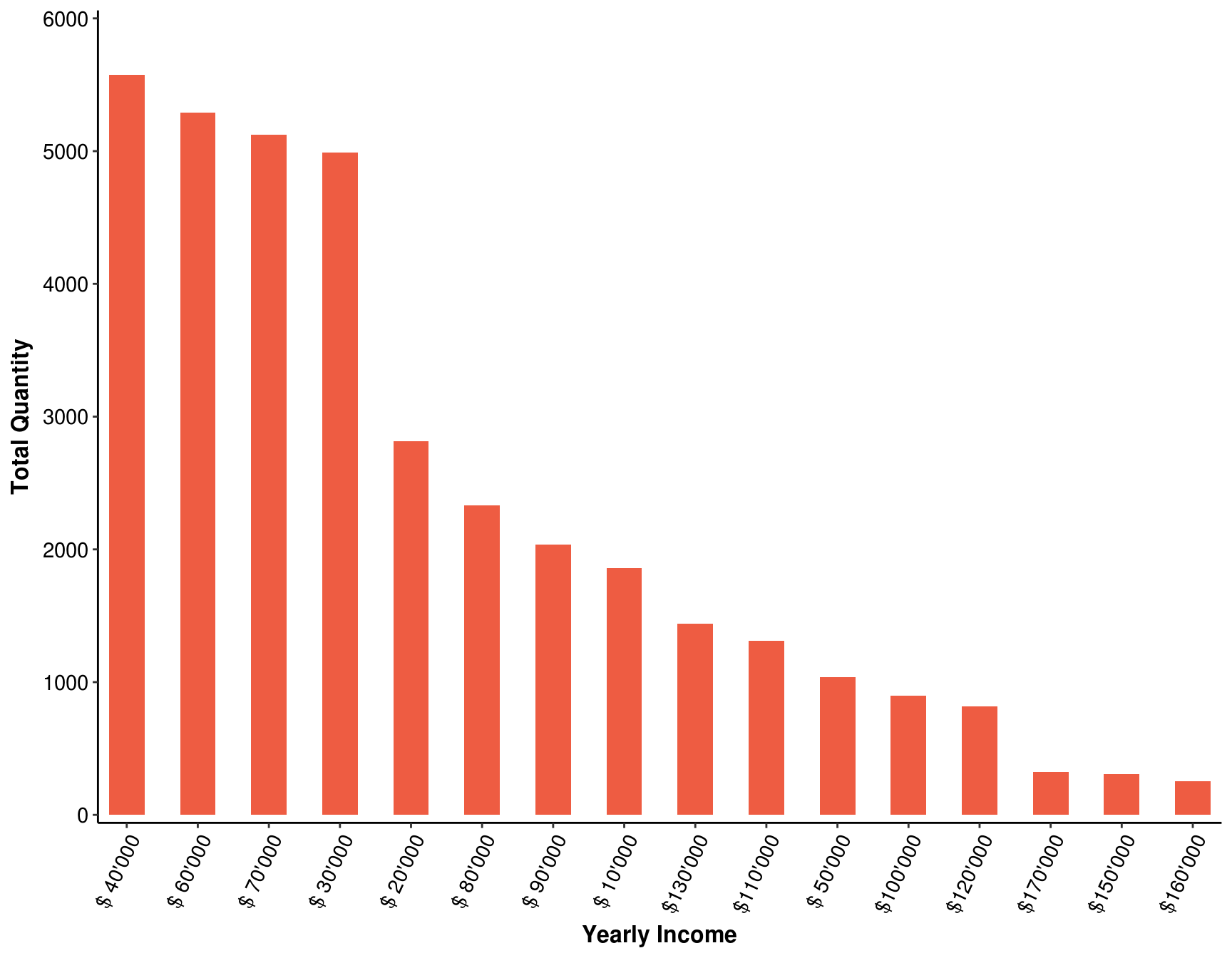

Answer:
1. $40000 2. $60000
3. $70`000

---

Now, remove the YearlyIncome field and replace it with the EnglishEducation field from the add_data tibble.

9.3 For those customers who bought bikes, what are the top two (bought the most quantity) education levels?

ans_3 <- my_data %>%
    select(`Customer ID`, `Order Quantity`, `Product Category`) %>%
    left_join(add_data %>%
                  select(Customer.ID, EnglishEducation), c("Customer ID" = "Customer.ID")) %>% 
    filter(`Product Category` == "Bikes") %>%
    group_by(EnglishEducation)%>%
    summarise(`Total Quantity` = sum(`Order Quantity`)) %>%
    arrange(desc(`Total Quantity`)) %>% 
    ungroup()
kable(ans_3)

EnglishEducation	Total Quantity
Bachelors	12201
Partial College	10389
Graduate Degree	6002
High School	5505
Partial High School	2314

ggplot(ans_3, aes(x = reorder(EnglishEducation, -`Total Quantity`),
                  y = `Total Quantity`, fill = EnglishEducation)) +
    geom_bar(stat = "identity", width = 0.5, show.legend = FALSE) +
    scale_y_continuous(breaks = seq(0, 15e4, by = 2e3), expand = c(0.01, 0)) +
    scale_fill_brewer(palette = "Dark2") +
    theme_classic() +
    theme(axis.title.x = element_blank(),
          axis.text = element_text(size = 13, colour = "black"),
          axis.title = element_text(size = 14, face = "bold"))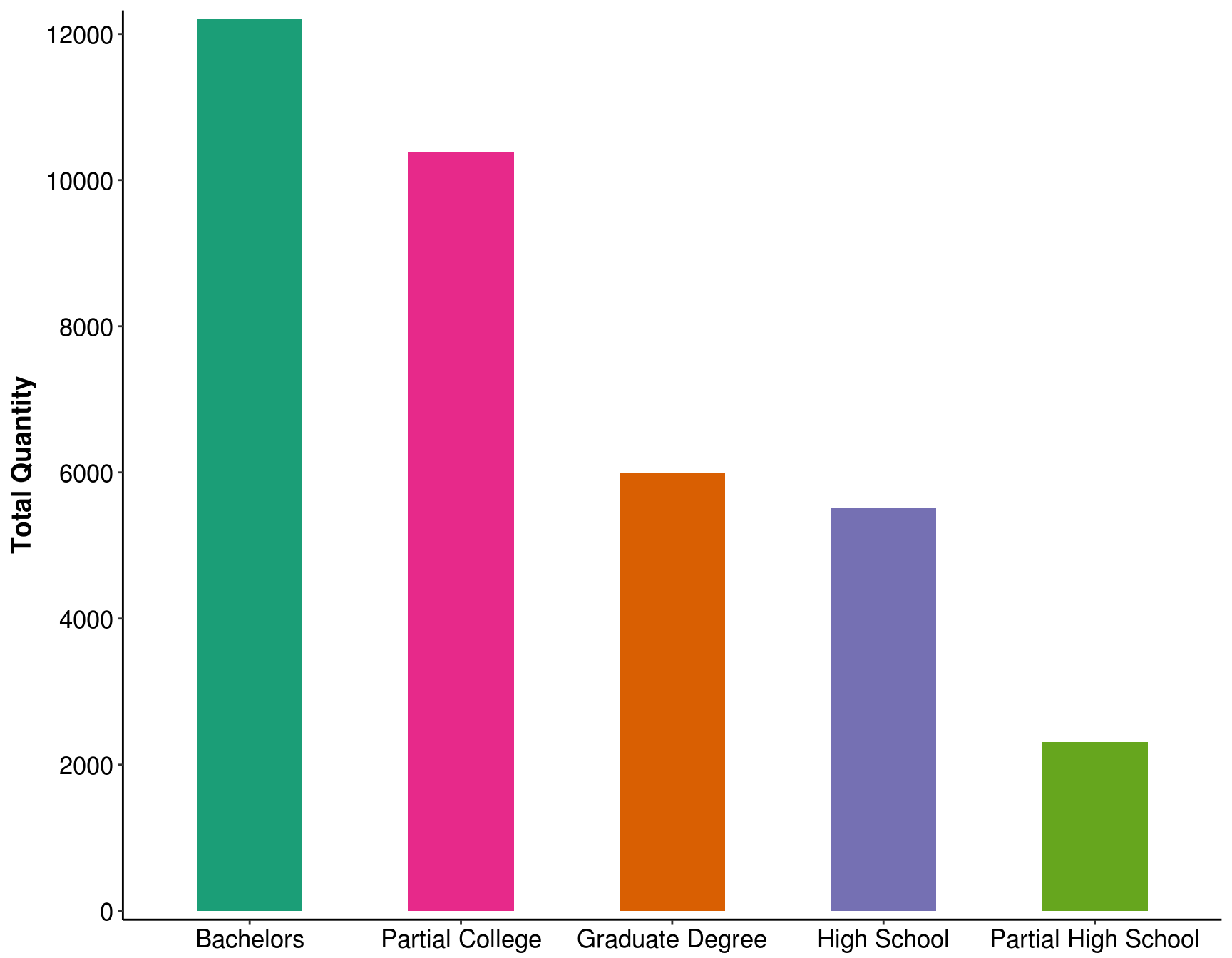

Answer:
1. Bachelors
2. Partial College

---

Lastly, remove the EnglishEducation field from the Rows and replace it with the HouseOwnerFlag field from the Customer_demographics table. Format the Sum of Order Quantity to show as Percentage of Grand Total with two decimal places.

9.4 What is the percentage of the customers who bought Bikes and are house owners?

ans_4 <- my_data %>%
    select(`Customer ID`, `Order Quantity`, `Product Category`) %>%
    left_join(add_data %>%
                  select(Customer.ID, HouseOwnerFlag), c("Customer ID" = "Customer.ID")) %>% 
    filter(`Product Category` == "Bikes") %>%
    group_by(HouseOwnerFlag) %>%
    summarise(Total = sum(`Order Quantity`)) %>%
    mutate(`Grand Total, %` = formatC(Total / sum(Total) * 100, digits = 2, format = "f") %>%
               as.numeric()) %>%
    arrange(desc(`Grand Total, %`)) %>% 
    ungroup()
kable(ans_4)

HouseOwnerFlag	Total	Grand Total, %
TRUE	25022	68.72
FALSE	11389	31.28

ggplot(ans_4, aes(x = "", y = Total / sum(Total), fill = HouseOwnerFlag)) +
    geom_bar(width = 1, stat = "identity", colour = "white", size = 0.7) +
    coord_polar(theta = "y") +
    labs(fill = "House\nOwner", x = NULL, y = NULL) +
    geom_text(aes(x = c(1.0, 1.1), y = c(0.35, 0.85), label = paste(`Grand Total, %`, "%")), size = 8) +
    scale_fill_brewer(palette = "Set2") +
    theme(panel.background = element_rect(fill = "white", color = "white"),
          plot.title = element_text(face = "bold", size = 16, hjust = 0.6),
          legend.title = element_text(face = "bold", colour = "black", size = 12),
          legend.text = element_text(size = 10, color = "black"),
          axis.text = element_blank(),
          axis.ticks = element_blank())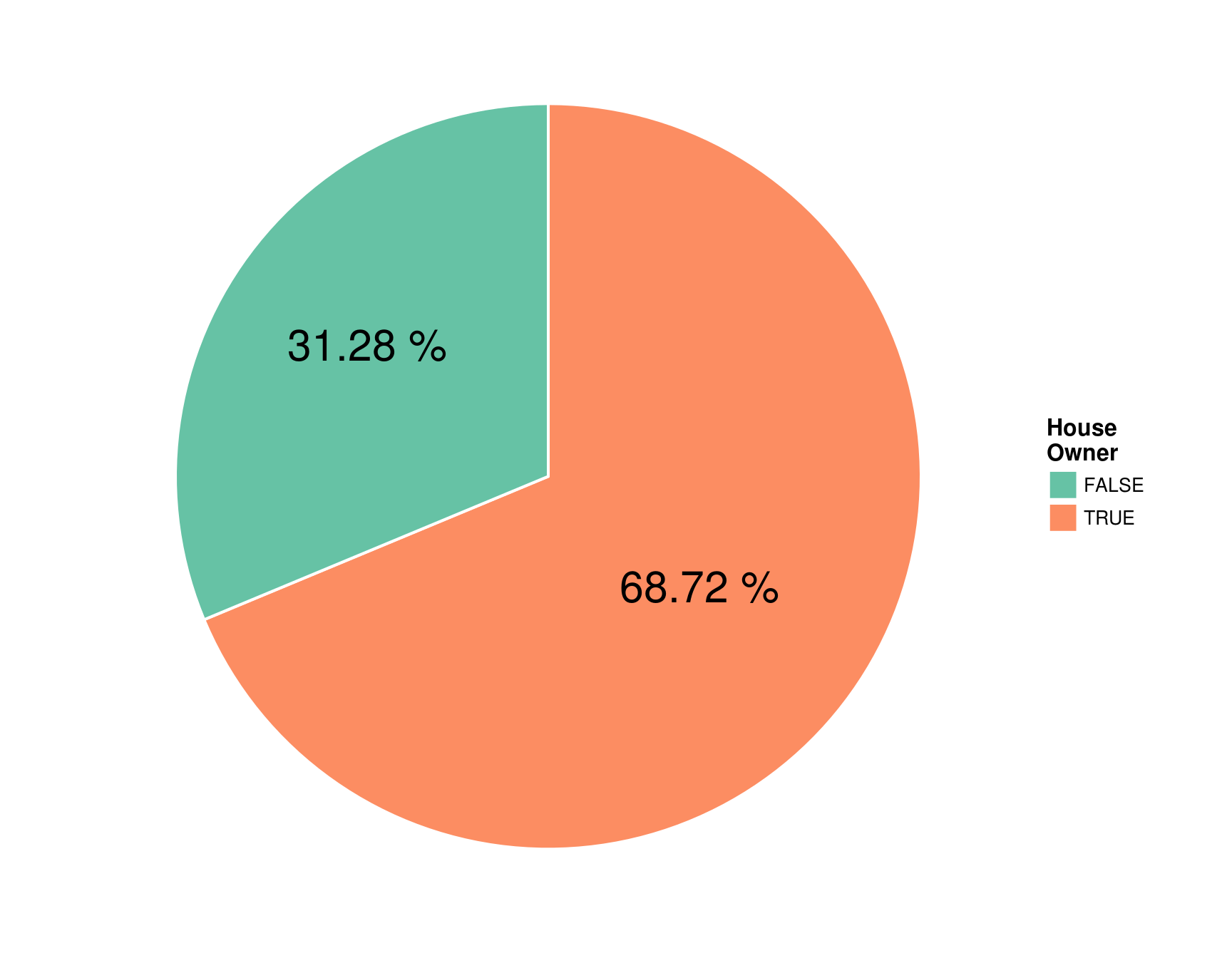

Answer: 68.72%