Chapter 6 Data: drill down
Scenario. Lucy was impressed with the dashboard you created. With the dashboard, she is able to narrow down her interest. Specifically, she is interested with the sales in Australia. She would like to perform simple profitability analysis on the product category and sub-category, for specific year. Furthermore, she wants to have the option of going deeper to product level.
Load libraries
library(tidyverse)
library(scales)
library(knitr)
Load data for Lab:
my_data <- readRDS("./data/processing/data4week3.rds")
str(my_data)
## Classes 'tbl_df', 'tbl' and 'data.frame': 113036 obs. of 19 variables:
## $ Date : POSIXct, format: "2013-11-26" "2015-11-26" ...
## $ Year : num 2013 2015 2014 2016 2014 ...
## $ Month : num 11 11 3 3 5 5 5 5 2 2 ...
## $ Customer ID : num 11019 11019 11039 11039 11046 ...
## $ Customer Age : num 19 19 49 49 47 47 47 47 35 35 ...
## $ Age Group : chr "Youth" "Youth" "Adults" "Adults" ...
## $ Customer Gender : chr "M" "M" "M" "M" ...
## $ Country : chr "Canada" "Canada" "Australia" "Australia" ...
## $ State : chr "British Columbia" "British Columbia" "New South Wales" "New South Wales" ...
## $ Product Category: chr "Accessories" "Accessories" "Accessories" "Accessories" ...
## $ Sub Category : chr "Bike Racks" "Bike Racks" "Bike Racks" "Bike Racks" ...
## $ Product : chr "Hitch Rack - 4-Bike" "Hitch Rack - 4-Bike" "Hitch Rack - 4-Bike" "Hitch Rack - 4-Bike" ...
## $ Frame Size : num NA NA NA NA NA NA NA NA NA NA ...
## $ Order Quantity : num 8 8 23 20 4 5 4 2 22 21 ...
## $ Unit Cost : num 45 45 45 45 45 45 45 45 45 45 ...
## $ Unit Price : num 120 120 120 120 120 120 120 120 120 120 ...
## $ Cost : num 360 360 1035 900 180 ...
## $ Revenue : num 950 950 2401 2088 418 ...
## $ Profit : num 590 590 1366 1188 238 ...Set common theme for charts:
common_theme <- theme_classic() +
    theme(axis.text.x = element_text(angle = 65, vjust = 1.0, hjust = 1.0),
          axis.text = element_text(size = 11, colour = "black"),
          axis.title = element_text(size = 12, face = "bold"))
Let’s start! Filter the pivot table for Australia and 2016, and answer the following questions.
6.1 Which subcategory sold the most quantity?
ans_1 <- my_data %>%
    filter(Country == "Australia", Year == 2016) %>%
    group_by(`Sub Category`) %>%
    summarise(Quantity = sum(`Order Quantity`)) %>%
    arrange(desc(Quantity))
kable(ans_1)| Sub Category | Quantity |
|---|---|
| Tires and Tubes | 26829 |
| Bottles and Cages | 14038 |
| Helmets | 9460 |
| Jerseys | 4353 |
| Caps | 3743 |
| Fenders | 2522 |
| Gloves | 2238 |
| Cleaners | 2052 |
| Hydration Packs | 1196 |
| Socks | 1005 |
| Road Bikes | 818 |
| Shorts | 813 |
| Vests | 808 |
| Mountain Bikes | 362 |
| Touring Bikes | 317 |
| Bike Racks | 221 |
| Bike Stands | 144 |
Find answer on chart:
ggplot(ans_1, aes(x = reorder(`Sub Category`, -Quantity), y = Quantity)) +
    geom_bar(stat = "identity", width = 0.5, fill="tomato2") +
    labs(x = "Sub Category") +
    scale_y_log10(breaks = c(10^(0:5), 3e4), expand = c(0.01, 0.01)) +
    common_theme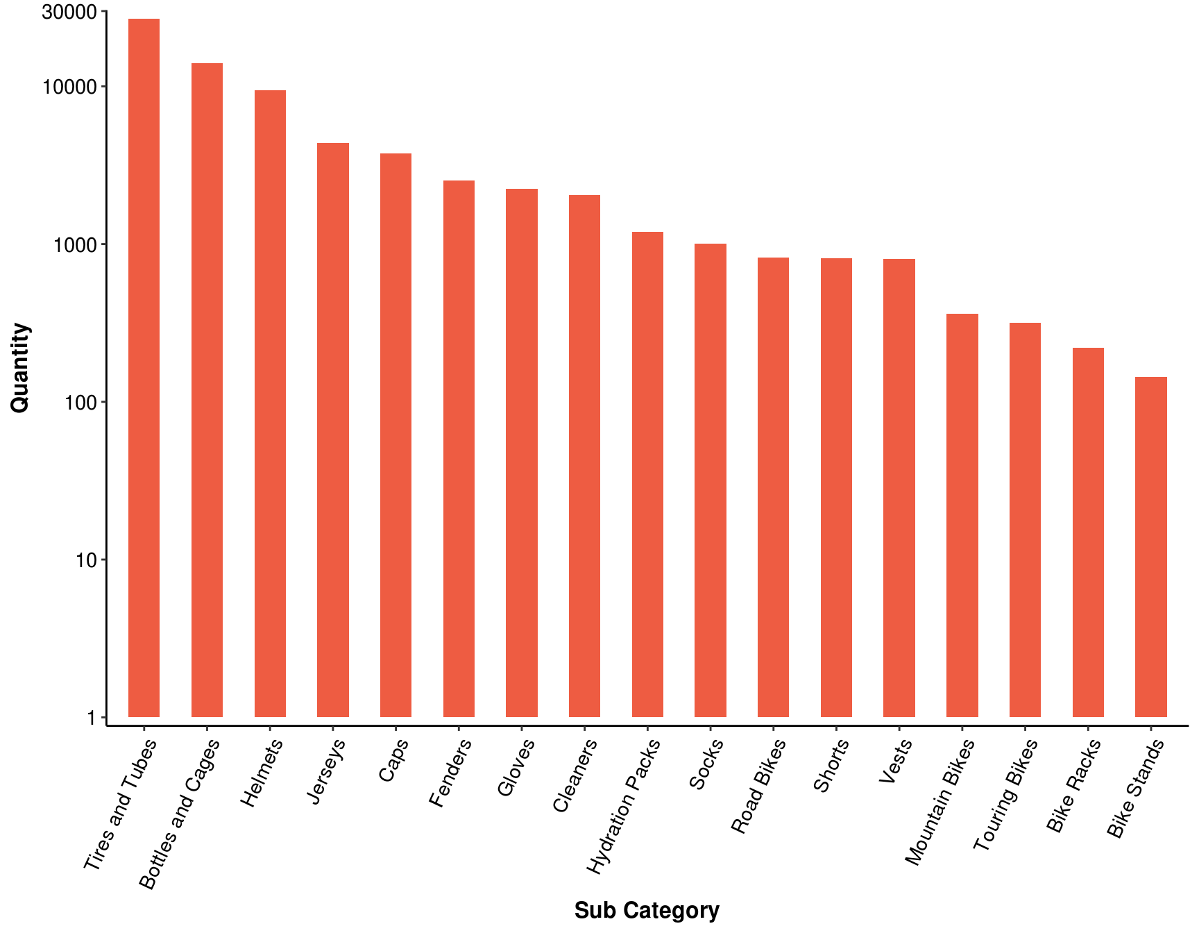
6.2 Which subcategory has the most revenue?
ans_2 <- my_data %>%
    filter(Country == "Australia", Year == 2016) %>%
    group_by(`Sub Category`) %>%
    summarise(`Total Revenue` = sum(Revenue)) %>%
    arrange(desc(`Total Revenue`))

ans_2 %>%
  mutate_at(vars(`Total Revenue`), funs(scales::comma)) %>%
kable()| Sub Category | Total Revenue |
|---|---|
| Road Bikes | 1,395,135 |
| Mountain Bikes | 679,575 |
| Touring Bikes | 407,333 |
| Helmets | 277,482 |
| Tires and Tubes | 235,712 |
| Jerseys | 192,735 |
| Bottles and Cages | 75,314 |
| Hydration Packs | 55,097 |
| Shorts | 47,562 |
| Fenders | 46,352 |
| Gloves | 45,198 |
| Vests | 43,392 |
| Caps | 28,349 |
| Bike Racks | 22,015 |
| Bike Stands | 19,326 |
| Cleaners | 13,802 |
| Socks | 7,604 |
Find answer on chart:
ggplot(ans_2, aes(x = reorder(`Sub Category`, -`Total Revenue`), y = `Total Revenue`)) +
    geom_bar(stat = "identity", width = 0.5, fill="tomato2") +
    labs(x = "Sub Category") +
    scale_y_log10(breaks = 10^(0:6), labels = scales::dollar, expand = c(0.01, 0)) +
    common_theme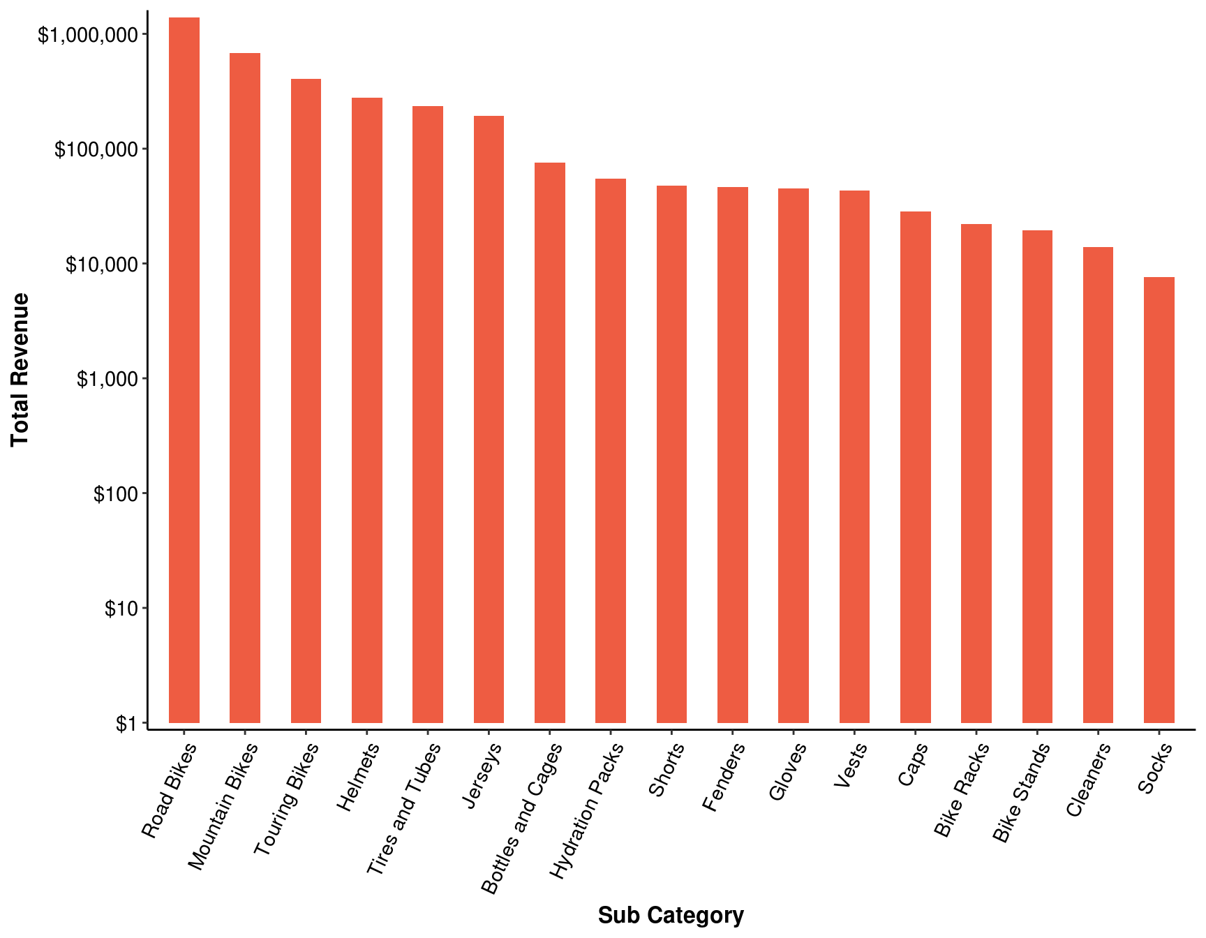
Now add a field Margin with the value derived from the Profit and Revenue column. Format the field as percentage with two decimal places. HINT: Margin = Profit / Revenue
6.3 What is the total margin for Australia in the year 2016?
ans_3 <- my_data %>%
    filter(Year == 2016) %>%
    group_by(Country) %>%
    summarise(`Margin` = sum(Profit) / sum(Revenue))
Find answer on chart:
ggplot(ans_3, aes(x = reorder(Country, -Margin), y = Margin, fill = Country)) +
    geom_bar(stat = "identity", width = 0.5, show.legend = FALSE) +
    labs(x = "Country") +
    scale_y_continuous(breaks = seq(0, .5, by = .1), expand = c(0.02, 0.0),
                       limits = c(0, .5), labels = scales::percent) +
    geom_text(aes(label = paste(formatC(`Margin` * 100, digits = 1, format = "f"), "%")),
              vjust = -0.5, colour = "black", fontface = "bold", size = 5) +
    theme_classic() +
    theme(axis.title = element_text(size = 12, face = "bold"),
          axis.text = element_text(size = 11, colour = "black"),
          axis.line.x = )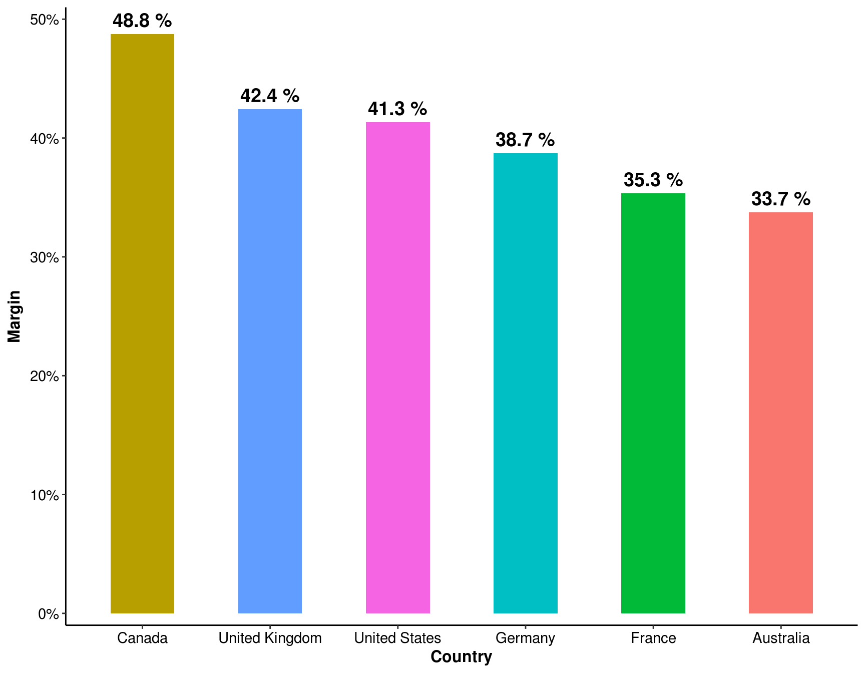
6.4 Using the same filters, which category has the lowest margin?
ans_4 <- my_data %>%
    filter(Country == "Australia", Year == 2016) %>%
    group_by(`Product Category`) %>%
    summarise(`Margin` = sum(Profit) / sum(Revenue))
Find answer on chart:
ggplot(ans_4, aes(x = reorder(`Product Category`, -`Margin`),
                  y = `Margin`, fill = `Product Category`)) +
    geom_bar(stat = "identity", width = 0.5, show.legend = FALSE) +
    labs(x = "Product Category") +
    scale_y_continuous(breaks = seq(0, .6, by = .1), expand = c(0.02, 0.0),
                       limits = c(0, .6), labels = scales::percent) +
    geom_text(aes(label = paste(formatC(`Margin` * 100, digits = 2, format = "f"), "%")),
              vjust = -0.5, colour = "black", fontface = "bold", size = 5) +
    theme_classic() +
    theme(axis.title = element_text(size = 12, face = "bold"),
          axis.text = element_text(size = 11, colour = "black"))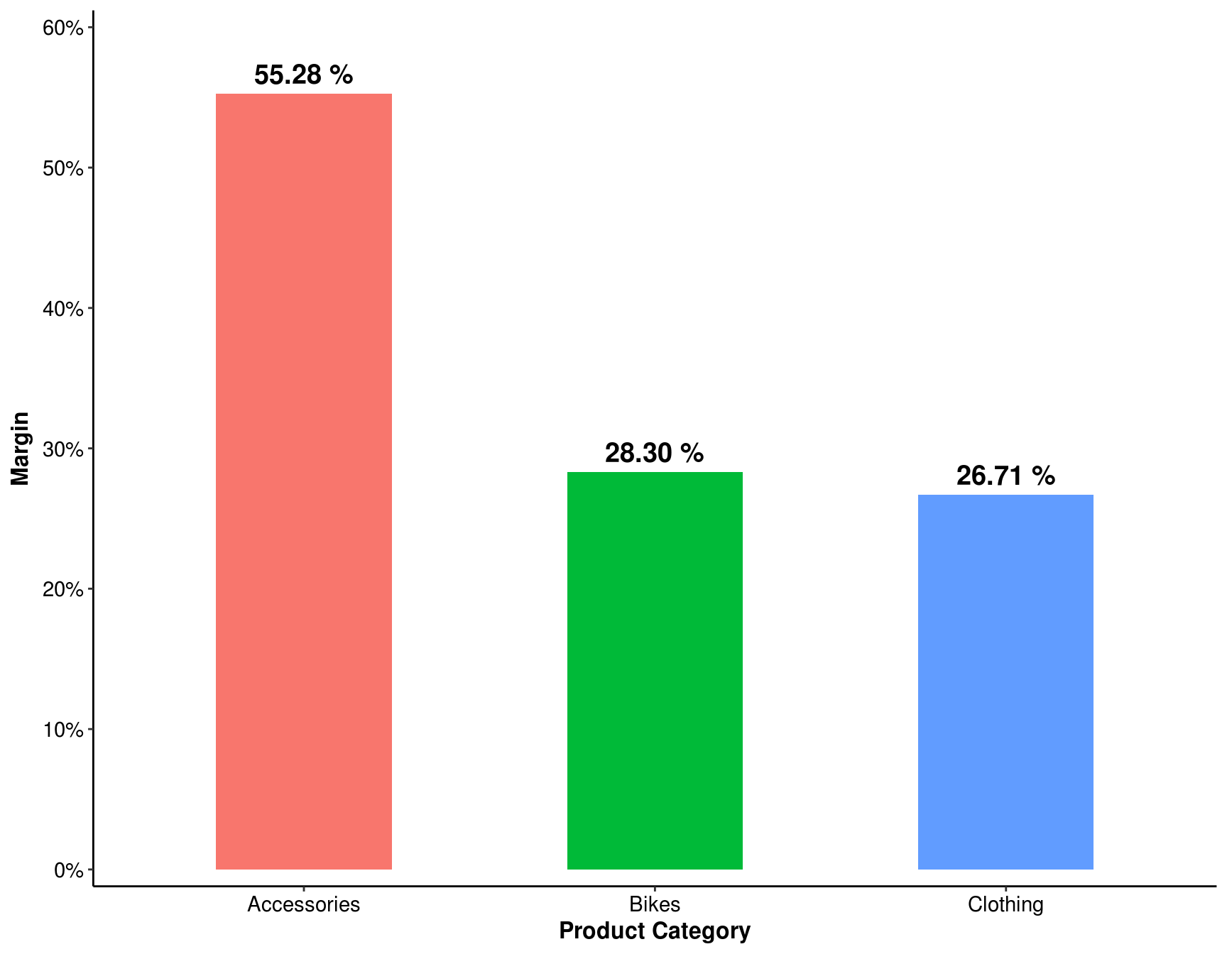
6.5 Which sub category has the lowest margin?
ans_5 <- my_data %>%
    filter(Country == "Australia", Year == 2016) %>%
    group_by(`Sub Category`) %>%
    summarise(`Margin` = sum(Profit) / sum(Revenue)) %>%
    arrange(Margin)

ans_5 %>%
  mutate_at(vars(Margin), funs(scales::percent)) %>%
kable()| Sub Category | Margin |
|---|---|
| Caps | 7.6% |
| Jerseys | 7.9% |
| Touring Bikes | 25.9% |
| Road Bikes | 26.2% |
| Mountain Bikes | 34.2% |
| Hydration Packs | 54.4% |
| Bottles and Cages | 54.8% |
| Bike Racks | 54.8% |
| Tires and Tubes | 54.9% |
| Vests | 55.3% |
| Cleaners | 55.4% |
| Gloves | 55.4% |
| Shorts | 55.6% |
| Helmets | 55.7% |
| Bike Stands | 56.0% |
| Fenders | 56.5% |
| Socks | 60.3% |
Find answer on chart:
ggplot(ans_5, aes(x = reorder(`Sub Category`, `Margin`),
                  y = `Margin`, fill = `Sub Category`)) +
    geom_bar(stat = "identity", width = 0.5, fill = "tomato2") +
    labs(x = "Sub Category") +
    scale_y_continuous(breaks = seq(0, .6, by = .1), expand = c(0.01, 0.0),
                       labels = scales::percent) +
    common_theme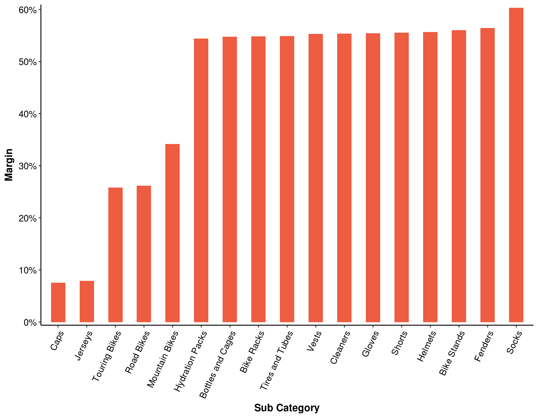
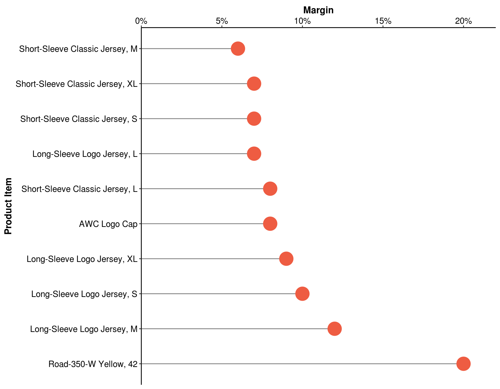
6.6 Which product has the least margin?
ans_6 <- my_data %>%
      filter(Country == "Australia", Year == 2016) %>%
      group_by(Product, `Sub Category`, `Product Category`) %>%
      summarise(Margin = formatC(sum(Profit) / sum(Revenue), digits = 2, format = "f") %>%
                    as.numeric()) %>%
      ungroup() %>%
      arrange(Margin) %>%
      top_n(-10)

ans_6 %>%
  mutate_at(vars(Margin), funs(scales::percent)) %>%
kable()| Product | Sub Category | Product Category | Margin |
|---|---|---|---|
| Short-Sleeve Classic Jersey, M | Jerseys | Clothing | 6% |
| Long-Sleeve Logo Jersey, L | Jerseys | Clothing | 7% |
| Short-Sleeve Classic Jersey, S | Jerseys | Clothing | 7% |
| Short-Sleeve Classic Jersey, XL | Jerseys | Clothing | 7% |
| AWC Logo Cap | Caps | Clothing | 8% |
| Short-Sleeve Classic Jersey, L | Jerseys | Clothing | 8% |
| Long-Sleeve Logo Jersey, XL | Jerseys | Clothing | 9% |
| Long-Sleeve Logo Jersey, S | Jerseys | Clothing | 10% |
| Long-Sleeve Logo Jersey, M | Jerseys | Clothing | 12% |
| Road-350-W Yellow, 42 | Road Bikes | Bikes | 20% |
Find answer on chart:
ggplot(ans_6, aes(y = reorder(Product, -`Margin`), x = Margin), fill = Product) +
    geom_segment(aes(yend = Product), xend = 0, colour = "grey50") +
    geom_point(size = 8, color = "tomato2") +
    labs(y = "Product Item") +
    scale_x_continuous(breaks = seq(0, .21, by = .05), labels = scales::percent,
                       limits = c(0, .22), expand = c(0, 0), position = "top") +
    theme_classic() +
    theme(axis.text = element_text(size = 11, colour = "black"),
          axis.title = element_text(size = 12, face = "bold"))